
What is the AI Learning process?
Before learning, let us see what is AI.
AI is defined as machine intelligence or the intelligence displayed by machines, as opposed to the natural intelligence displayed by humans. The term AI is often used to describe machines that mimic human cognitive functions such as learning, understanding, reasoning, or problem-solving. Artificial Intelligence (AI) has become one of the most sought-after capabilities in business and trades these days. AI is already being increasingly implemented by the world’s largest corporations due to its wide-ranging benefits in reducing human overhead, increasing efficiency, and making processes faster.
If we talk further, everyone’s future will depend on AI. So why can’t we make our career in this? I Will guide you through AI step by step—the easiest way to learn artificial intelligence. You have to enrol in an online program through the new good e-learning platform, I have given a link below. By registering there you can become a part of the training. To get an Artificial Intelligence AI knowledge course, you do not need to take fees and admission anywhere. You will get everything for free. First, you have to understand the learning module by yourself, then you have to see how it works, then after using it yourself, you can apply for the job to work in the company.
About Artificial Intelligence
Artificial Intelligence: These are designed for specific people, we now call them developers. But it is not that only engineers can use it. Even those who do not know engineering can use it—people who want to focus on coding who have never done any programming or engineering before. So no problem. We can also learn it. Therefore, I request all of you to understand the Artificial Intelligence certification, please do it carefully, otherwise, it will be a loss for you.
Machine Learning Algorithms
A machine learning algorithm refers to a program code (mathematics or program logic) that enables professionals to study, analyze, understand, and explore large complex datasets. Every algorithm follows a series of instructions to accomplish the purpose of making predictions or classifying information by learning, establishing, and discovering patterns embedded in the data. There are some important components inside it. It has to be confirmed. So you will have to practice the points given below.

Objectives
- They are generally depending on some issues of machine learning techniques and algorithms used in AI.
- Algorithms covered – Linear Regression, Logistic Regression, Naive Bayes, KNN, Random Forest, etc.
- Need to know both the theory and implementation of machine learning algorithms in R and Python.
Fundamentals of AI
· Statistical Fundamentals
· Programming Fundamentals.
· Database management fundamentals.
Best Machine Learning Algorithms Tools
Machine learning does all the work as a task and its ability is very good i.e. work faster. It does all the work in a certain amount of time. All such intelligent systems work on machine learning algorithms. We see that in data science, each machine learning algorithm handles a specific problem, i.e. it performs its intended function. In some cases, professionals choose a combination of these algorithms because a single algorithm cannot solve a specific problem, so a process is determined at each step. All algorithms are working on this. Each algorithm is assigned, so which algorithm does what works?
Linear regression
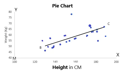
It is used to estimate actual values based on a continuous variable. Linear regression gives the relationship between the input (x) and the output variable (y), also known as the independent and dependent variables.
As shown in the figure below, linear regression is similar to machine learning, where the relationship between the independent and dependent variables is established by fitting a regression line. This line has a mathematical representation given by the linear equation y = mx + c, where y represents the dependent variable, m = slope, x = independent variable, and b = intercept. Thus linear regression is used.
R Code
To use R Code – the cooch command is required. I have given that command below and how to use it has also been given.

					#Load Train and Test datasets #Identify feature and response variable(s) and values must be numeric and numpy arrays

 x_train <-input_variables_values_training_datasets

y_train <- target_variables_values_training_datasets

x_test <- input_variables_values_test_datasets

x <- cbind(x_train,y_train) # Train the model using the training sets and check score

linear <- lm(y_train ~ ., data = x)

summary(linear)

#Predict Output

predicted= predict(linear,x_test)
Python
# importing required libraries
import pandas as pd
from sklearn.linear_model import LinearRegression
from sklearn.metrics import mean_squared_error

# read the train and test dataset
train_data = pd.read_csv('train.csv')
test_data = pd.read_csv('test.csv')

print(train_data.head())

# shape of the dataset
print('\nShape of training data :',train_data.shape)
print('\nShape of testing data :',test_data.shape)

# Now, we need to predict the missing target variable in the test data
# target variable - Item_Outlet_Sales

# seperate the independent and target variable on training data
train_x = train_data.drop(columns=['Item_Outlet_Sales'],axis=1)
train_y = train_data['Item_Outlet_Sales']

# seperate the independent and target variable on training data
test_x = test_data.drop(columns=['Item_Outlet_Sales'],axis=1)
test_y = test_data['Item_Outlet_Sales']

'''
Create the object of the Linear Regression model
You can also add other parameters and test your code here
Some parameters are : fit_intercept and normalize
Documentation of sklearn LinearRegression:

https://scikit-learn.org/stable/modules/generated/sklearn.linear_model.LinearRegression.html

 '''
model = LinearRegression()

# fit the model with the training data
model.fit(train_x,train_y)

# coefficeints of the trained model
print('\nCoefficient of model :', model.coef_)

# intercept of the model
print('\nIntercept of model',model.intercept_)

# predict the target on the test dataset
predict_train = model.predict(train_x)
print('\nItem_Outlet_Sales on training data',predict_train)

# Root Mean Squared Error on training dataset
rmse_train = mean_squared_error(train_y,predict_train)**(0.5)
print('\nRMSE on train dataset : ', rmse_train)

# predict the target on the testing dataset
predict_test = model.predict(test_x)
print('\nItem_Outlet_Sales on test data',predict_test)

# Root Mean Squared Error on testing dataset
rmse_test = mean_squared_error(test_y,predict_test)**(0.5)
print('\nRMSE on test dataset : ', rmse_test)
Logistic Regression
This task is to estimate positive and negative. In logistic regression, the dependent variable is of binary type (dichotomous). Thus, the binary outcomes of logistic regression facilitate faster decision-making as you only need to choose one of two options. Logistic regression is used in predictive analysis where relevant data is fit to a logit function predicting the probability of an event. It is also called logit regression.
Formula: y = e^(b0 + b1*x) / (1 + e^(b0 + b1*x))
R Code
					x <- cbind(x_train,y_train)
# Train the model using the training sets and check score
logistic <- glm(y_train ~ ., data = x,family='binomial')
summary(logistic)
#Predict Output
predicted= predict(logistic,x_test)
Python
# importing required libraries
import pandas as pd
from sklearn.linear_model import LogisticRegression
from sklearn.metrics import accuracy_score

# read the train and test dataset
train_data = pd.read_csv('train-data.csv')
test_data = pd.read_csv('test-data.csv')


print(train_data.head())

# shape of the dataset
print('Shape of training data :',train_data.shape)
print('Shape of testing data :',test_data.shape)

# Now, we need to predict the missing target variable in the test data
# target variable - Survived

# seperate the independent and target variable on training data
train_x = train_data.drop(columns=['Survived'],axis=1)
train_y = train_data['Survived']

# seperate the independent and target variable on testing data
test_x = test_data.drop(columns=['Survived'],axis=1)
test_y = test_data['Survived']

'''
Create the object of the Logistic Regression model
You can also add other parameters and test your code here
Some parameters are : fit_intercept and penalty
Documentation of sklearn LogisticRegression:

https://scikit-learn.org/stable/modules/generated/sklearn.linear_model.LogisticRegression.html

 '''
model = LogisticRegression()

# fit the model with the training data
model.fit(train_x,train_y)

# coefficeints of the trained model
print('Coefficient of model :', model.coef_)

# intercept of the model
print('Intercept of model',model.intercept_)

# predict the target on the train dataset
predict_train = model.predict(train_x)
print('Target on train data',predict_train)

# Accuray Score on train dataset
accuracy_train = accuracy_score(train_y,predict_train)
print('accuracy_score on train dataset : ', accuracy_train)

# predict the target on the test dataset
predict_test = model.predict(test_x)
print('Target on test data',predict_test)

# Accuracy Score on test dataset
accuracy_test = accuracy_score(test_y,predict_test)
print('accuracy_score on test dataset : ', accuracy_test)
Decision Tree
Decision Tree Algorithms can predict the best possible option based on a mathematical model and are also useful in brainstorming a particular decision. It is a type of supervised learning algorithm mainly used for classification problems. Characteristically, it works for both categorical and continuous dependent variables. In this algorithm, we divide the population into two or more homogeneous sets. This algorithm creates a tree-like structure that is used for classification problems.
For more information, you can understand the decision tree below.

R Code
					library(rpart)
x <- cbind(x_train,y_train)
# grow tree
fit <- rpart(y_train ~ ., data = x,method="class")
summary(fit)
#Predict Output
predicted= predict(fit,x_test)
Python
# importing required libraries
import pandas as pd
from sklearn.tree import DecisionTreeClassifier
from sklearn.metrics import accuracy_score

# read the train and test dataset
train_data = pd.read_csv('train-data.csv')
test_data = pd.read_csv('test-data.csv')

# shape of the dataset
print('Shape of training data :',train_data.shape)
print('Shape of testing data :',test_data.shape)

# Now, we need to predict the missing target variable in the test data
# target variable - Survived

# seperate the independent and target variable on training data
train_x = train_data.drop(columns=['Survived'],axis=1)
train_y = train_data['Survived']

# seperate the independent and target variable on testing data
test_x = test_data.drop(columns=['Survived'],axis=1)
test_y = test_data['Survived']

'''
Create the object of the Decision Tree model
You can also add other parameters and test your code here
Some parameters are : max_depth and max_features
Documentation of sklearn DecisionTreeClassifier:

https://scikit-learn.org/stable/modules/generated/sklearn.tree.DecisionTreeClassifier.html

 '''
model = DecisionTreeClassifier()

# fit the model with the training data
model.fit(train_x,train_y)

# depth of the decision tree
print('Depth of the Decision Tree :', model.get_depth())

# predict the target on the train dataset
predict_train = model.predict(train_x)
print('Target on train data',predict_train)

# Accuray Score on train dataset
accuracy_train = accuracy_score(train_y,predict_train)
print('accuracy_score on train dataset : ', accuracy_train)

# predict the target on the test dataset
predict_test = model.predict(test_x)
print('Target on test data',predict_test)

# Accuracy Score on test dataset
accuracy_test = accuracy_score(test_y,predict_test)
print('accuracy_score on test dataset : ', accuracy_test)
Support vector machines (SVM)
This is a classification method. Support vector machine algorithms are used to perform both classification and regression tasks. In the SVM algorithm, as taught in school—plot each data item as a point in an n-dimensional space where n is the number of your features, each feature value is the value of a particular index.
Simply put, SVMs represent coordinates for individual observations. In data classification process, these are popular machine learning classifiers used in applications such as facial expression classification, text classification, steganography detection in digital images, speech recognition and others. Thus SVM is expected to be of great value.

R Code
					library(e1071)
x <- cbind(x_train,y_train)
# Fitting model
fit <-svm(y_train ~ ., data = x)
summary(fit)
#Predict Output
predicted= predict(fit,x_test)
Python
# importing required libraries
import pandas as pd
from sklearn.svm import SVC
from sklearn.metrics import accuracy_score

# read the train and test dataset
train_data = pd.read_csv('train-data.csv')
test_data = pd.read_csv('test-data.csv')

# shape of the dataset
print('Shape of training data :',train_data.shape)
print('Shape of testing data :',test_data.shape)

# Now, we need to predict the missing target variable in the test data
# target variable - Survived

# seperate the independent and target variable on training data
train_x = train_data.drop(columns=['Survived'],axis=1)
train_y = train_data['Survived']

# seperate the independent and target variable on testing data
test_x = test_data.drop(columns=['Survived'],axis=1)
test_y = test_data['Survived']

'''
Create the object of the Support Vector Classifier model
You can also add other parameters and test your code here
Some parameters are : kernal and degree
Documentation of sklearn Support Vector Classifier:

https://scikit-learn.org/stable/modules/generated/sklearn.svm.SVC.html

 '''
model = SVC()

# fit the model with the training data
model.fit(train_x,train_y)

# predict the target on the train dataset
predict_train = model.predict(train_x)
print('Target on train data',predict_train)

# Accuray Score on train dataset
accuracy_train = accuracy_score(train_y,predict_train)
print('accuracy_score on train dataset : ', accuracy_train)

# predict the target on the test dataset
predict_test = model.predict(test_x)
print('Target on test data',predict_test)

# Accuracy Score on test dataset
accuracy_test = accuracy_score(test_y,predict_test)
print('accuracy_score on test dataset : ', accuracy_test)
Naive Bayes
Naive Bayes refers to probabilistic machine learning algorithms based on Bayesian probability models and used to solve nomenclature problems. In simple terms, a naïve Bayes classifier assumes that the presence of a particular full-length in matriculation is unrelated to the presence of any other feature. Naïve Bayesian models are easy to construct and particularly useful for very large data sets. Along with naivety, Naive Bayes is known to outperform plane the most sophisticated nomenclature methods. This implies that the vital theorizing of the algorithm is that the features under consideration are self-sustaining of each other and a transpiration in the value of one does not stupefy the value of the other.
For example, consider a cricket wittiness if it is red, round, 7.1-7.26 cm in diameter and has a mass of 156-163 grams. All these characteristics may be interdependent, while each contributes to the probability of stuffing a cricket ball. This is why the algorithm is tabbed ‘naive’.
Bayes’ Theorem:
P (X|Y) = (P (Y|X) x P (X)) /P (Y)
Mathematical representation.
If X, Y = probable event, P (X) = probability that X is true, P(X|Y) = provisionary probability that X is true if Y is true.
R Code
					library(e1071)
x <- cbind(x_train,y_train)
# Fitting model
fit <-naiveBayes(y_train ~ ., data = x)
summary(fit)
#Predict Output
predicted= predict(fit,x_test)
Python
# importing required libraries
import pandas as pd
from sklearn.naive_bayes import GaussianNB
from sklearn.metrics import accuracy_score

# read the train and test dataset
train_data = pd.read_csv('train-data.csv')
test_data = pd.read_csv('test-data.csv')

# shape of the dataset
print('Shape of training data :',train_data.shape)
print('Shape of testing data :',test_data.shape)

# Now, we need to predict the missing target variable in the test data
# target variable - Survived

# seperate the independent and target variable on training data
train_x = train_data.drop(columns=['Survived'],axis=1)
train_y = train_data['Survived']

# seperate the independent and target variable on testing data
test_x = test_data.drop(columns=['Survived'],axis=1)
test_y = test_data['Survived']

'''
Create the object of the Naive Bayes model
You can also add other parameters and test your code here
Some parameters are : var_smoothing
Documentation of sklearn GaussianNB:

https://scikit-learn.org/stable/modules/generated/sklearn.naive_bayes.GaussianNB.html

 '''
model = GaussianNB()

# fit the model with the training data
model.fit(train_x,train_y)

# predict the target on the train dataset
predict_train = model.predict(train_x)
print('Target on train data',predict_train)

# Accuray Score on train dataset
accuracy_train = accuracy_score(train_y,predict_train)
print('accuracy_score on train dataset : ', accuracy_train)

# predict the target on the test dataset
predict_test = model.predict(test_x)
print('Target on test data',predict_test)

# Accuracy Score on test dataset
accuracy_test = accuracy_score(test_y,predict_test)
print('accuracy_score on test dataset : ', accuracy_test)
KNN Algorithms
K Nearest Neighbors (KNN) is a simple, intuitive and versatile algorithm used for both classification and regression tasks in machine learning. Despite its simplicity, Naive Bays lends itself well to a variety of real-world applications. The K Nearestighbours (KNN) algorithm is used for both classification and regression problems. It stores all known use cases and classifies new use cases (or data points) into different classes. KNN is a valuable algorithm in many contexts, especially when relationships in data are not easily captured by more complex models. It is often used as a baseline or as part of an addition to a machine-learning pipeline.

R Code
					library(knn)
x <- cbind(x_train,y_train)
# Fitting model
fit <-knn(y_train ~ ., data = x,k=5)
summary(fit)
#Predict Output
predicted= predict(fit,x_test)
Python
					# importing required libraries
import pandas as pd
from sklearn.neighbors import KNeighborsClassifier
from sklearn.metrics import accuracy_score

# read the train and test dataset
train_data = pd.read_csv('train-data.csv')
test_data = pd.read_csv('test-data.csv')

# shape of the dataset
print('Shape of training data :',train_data.shape)
print('Shape of testing data :',test_data.shape)

# Now, we need to predict the missing target variable in the test data
# target variable - Survived

# seperate the independent and target variable on training data
train_x = train_data.drop(columns=['Survived'],axis=1)
train_y = train_data['Survived']

# seperate the independent and target variable on testing data
test_x = test_data.drop(columns=['Survived'],axis=1)
test_y = test_data['Survived']

'''
Create the object of the K-Nearest Neighbor model
You can also add other parameters and test your code here
Some parameters are : n_neighbors, leaf_size
Documentation of sklearn K-Neighbors Classifier:

https://scikit-learn.org/stable/modules/generated/sklearn.neighbors.KNeighborsClassifier.html

 '''
model = KNeighborsClassifier()

# fit the model with the training data
model.fit(train_x,train_y)

# Number of Neighbors used to predict the target
print('\nThe number of neighbors used to predict the target : ',model.n_neighbors)

# predict the target on the train dataset
predict_train = model.predict(train_x)
print('\nTarget on train data',predict_train)

# Accuray Score on train dataset
accuracy_train = accuracy_score(train_y,predict_train)
print('accuracy_score on train dataset : ', accuracy_train)

# predict the target on the test dataset
predict_test = model.predict(test_x)
print('Target on test data',predict_test)

# Accuracy Score on test dataset
accuracy_test = accuracy_score(test_y,predict_test)
print('accuracy_score on test dataset : ', accuracy_test)
K-Means
K-Means is a popular clustering algorithm used in unsupervised machine learning. In this algorithm, you classify datasets into clusters (K clusters) where the data points within one set remain homogenous, and the data points from two different clusters remain heterogeneous. The algorithm iteratively refines the assignment of data points to clusters until a convergence criterion is met.
R Code
					library(cluster)
fit <- kmeans(X, 3) # 5 cluster solution
Python
					# importing required libraries
import pandas as pd
from sklearn.cluster import KMeans

# read the train and test dataset
train_data = pd.read_csv('train-data.csv')
test_data = pd.read_csv('test-data.csv')

# shape of the dataset
print('Shape of training data :',train_data.shape)
print('Shape of testing data :',test_data.shape)

# Now, we need to divide the training data into differernt clusters
# and predict in which cluster a particular data point belongs.

'''
Create the object of the K-Means model
You can also add other parameters and test your code here
Some parameters are : n_clusters and max_iter
Documentation of sklearn KMeans:

https://scikit-learn.org/stable/modules/generated/sklearn.cluster.KMeans.html
 '''

model = KMeans()

# fit the model with the training data
model.fit(train_data)

# Number of Clusters
print('\nDefault number of Clusters : ',model.n_clusters)

# predict the clusters on the train dataset
predict_train = model.predict(train_data)
print('\nCLusters on train data',predict_train)

# predict the target on the test dataset
predict_test = model.predict(test_data)
print('Clusters on test data',predict_test)

# Now, we will train a model with n_cluster = 3
model_n3 = KMeans(n_clusters=3)

# fit the model with the training data
model_n3.fit(train_data)

# Number of Clusters
print('\nNumber of Clusters : ',model_n3.n_clusters)

# predict the clusters on the train dataset
predict_train_3 = model_n3.predict(train_data)
print('\nCLusters on train data',predict_train_3)

# predict the target on the test dataset
predict_test_3 = model_n3.predict(test_data)
print('Clusters on test data',predict_test_3)
Random forest
Random Forest is an ensemble learning method that works by generating multiple visualization trees during training. The “randomness” of a random forest comes from using random subsamples of the training data and subsets of random features to train each tree. It is a supervised machine learning algorithm where variegated visualization trees are generated on variegated samples during training. These algorithms help to estimate missing data. Random forest is a trademarked term for ensemble learning of visualization trees. In a random forest, we have a hodgepodge of visualization trees (also known as a “big forest”). It is that.

R Code
					library(cluster)
fit <- kmeans(X, 3) # 5 cluster solution
Python
					# importing required libraries
import pandas as pd
from sklearn.cluster import KMeans

# read the train and test dataset
train_data = pd.read_csv('train-data.csv')
test_data = pd.read_csv('test-data.csv')

# shape of the dataset
print('Shape of training data :',train_data.shape)
print('Shape of testing data :',test_data.shape)

# Now, we need to divide the training data into differernt clusters
# and predict in which cluster a particular data point belongs.

'''
Create the object of the K-Means model
You can also add other parameters and test your code here
Some parameters are : n_clusters and max_iter
Documentation of sklearn KMeans:

https://scikit-learn.org/stable/modules/generated/sklearn.cluster.KMeans.html
 '''

model = KMeans()

# fit the model with the training data
model.fit(train_data)

# Number of Clusters
print('\nDefault number of Clusters : ',model.n_clusters)

# predict the clusters on the train dataset
predict_train = model.predict(train_data)
print('\nCLusters on train data',predict_train)

# predict the target on the test dataset
predict_test = model.predict(test_data)
print('Clusters on test data',predict_test)

# Now, we will train a model with n_cluster = 3
model_n3 = KMeans(n_clusters=3)

# fit the model with the training data
model_n3.fit(train_data)

# Number of Clusters
print('\nNumber of Clusters : ',model_n3.n_clusters)

# predict the clusters on the train dataset
predict_train_3 = model_n3.predict(train_data)
print('\nCLusters on train data',predict_train_3)

# predict the target on the test dataset
predict_test_3 = model_n3.predict(test_data)
print('Clusters on test data',predict_test_3)
Dimensionality Reduction Algorithms
Dimensionality reduction techniques are used in machine learning and data analysis to reduce the number of input variables or features in a dataset while preserving as much relevant information as possible. This can be beneficial for various reasons, such as speeding up training time, mitigating the curse of dimensionality, and gaining insights into the underlying structure of the data.
R Code
					library(stats)
pca <- princomp(train, cor = TRUE)
train_reduced  <- predict(pca,train)
test_reduced  <- predict(pca,test)
Python
					# importing required libraries
import pandas as pd
from sklearn.decomposition import PCA
from sklearn.linear_model import LinearRegression
from sklearn.metrics import mean_squared_error

# read the train and test dataset
train_data = pd.read_csv('train.csv')
test_data = pd.read_csv('test.csv')

# view the top 3 rows of the dataset
print(train_data.head(3))

# shape of the dataset
print('\nShape of training data :',train_data.shape)
print('\nShape of testing data :',test_data.shape)

# Now, we need to predict the missing target variable in the test data
# target variable - Survived

# seperate the independent and target variable on training data
# target variable - Item_Outlet_Sales
train_x = train_data.drop(columns=['Item_Outlet_Sales'],axis=1)
train_y = train_data['Item_Outlet_Sales']

# seperate the independent and target variable on testing data
test_x = test_data.drop(columns=['Item_Outlet_Sales'],axis=1)
test_y = test_data['Item_Outlet_Sales']

print('\nTraining model with {} dimensions.'.format(train_x.shape[1]))

# create object of model
model = LinearRegression()

# fit the model with the training data
model.fit(train_x,train_y)

# predict the target on the train dataset
predict_train = model.predict(train_x)

# Accuray Score on train dataset
rmse_train = mean_squared_error(train_y,predict_train)**(0.5)
print('\nRMSE on train dataset : ', rmse_train)

# predict the target on the test dataset
predict_test = model.predict(test_x)

# Accuracy Score on test dataset
rmse_test = mean_squared_error(test_y,predict_test)**(0.5)
print('\nRMSE on test dataset : ', rmse_test)

# create the object of the PCA (Principal Component Analysis) model
# reduce the dimensions of the data to 12
'''
You can also add other parameters and test your code here
Some parameters are : svd_solver, iterated_power
Documentation of sklearn PCA:

https://scikit-learn.org/stable/modules/generated/sklearn.decomposition.PCA.html
'''
model_pca = PCA(n_components=12)

new_train = model_pca.fit_transform(train_x)
new_test  = model_pca.fit_transform(test_x)

print('\nTraining model with {} dimensions.'.format(new_train.shape[1]))

# create object of model
model_new = LinearRegression()

# fit the model with the training data
model_new.fit(new_train,train_y)

# predict the target on the new train dataset
predict_train_pca = model_new.predict(new_train)

# Accuray Score on train dataset
rmse_train_pca = mean_squared_error(train_y,predict_train_pca)**(0.5)
print('\nRMSE on new train dataset : ', rmse_train_pca)

# predict the target on the new test dataset
predict_test_pca = model_new.predict(new_test)

# Accuracy Score on test dataset
rmse_test_pca = mean_squared_error(test_y,predict_test_pca)**(0.5)
print('\nRMSE on new test dataset : ', rmse_test_pca)
Course
Very Important Notice:
Artificial Intelligence: A Comprehensive Overview Explains what Artificial Intelligence (AI) is and what the various AI concepts represent. As a result, your vocabulary will expand and you will be able to communicate with other AI-related programmers. However, this institute does not provide a domain specialization feature in its AI courses.
1. Learnbay(Recommended)

The Learnbay’s Artificial Intelligence Certification Training is one of my personal favorites considering the undertow format for beginners focuses not only on towers the essentials, but also on learning the nonflexible concepts as you understand the techniques, qualify projects, and get certified by instructors. I can moreover tell you that it is very good.
2. Artificial Intelligence A-Z: Udemy

This undertow will show you how to use Data Science, Machine Learning, and Deep Learning to construct strong AI for real-world applications such as vibration Breakout, passing a level in Doom, and creating reasoning for self-driving cars. However, it doesn’t have real-time projects and Course duration is 9 months.
Finally, I would like to recommend Learnbay for working pros and Edureka for freshers. Coursera is suggested exclusively for those who want to learn just to know more, not with a career up-gradation target.